Number Theoretic Transform
Number Theoretic Transform(NTT) is an efficient algorithm for polynomial multiplication, akin to the Fast Fourier Transform (FFT). It operates in finite fields, making it particularly valuable in cryptography and coding theory, where it enables rapid computations on large numbers and polynomials. For the purposes of this document, polynomials are assumed to be defined over finite fields by default.
Polynomial Multiplication
Let's consider two polynomials:
The product can be expressed as:
By expanding, we find:
In a programming context, we can represent polynomials as follows:
= coefficient of degree term of polynomial
Using the distributive property, the runtime for multiplying two polynomials of degree is .However, is there a more efficient method?
Polynomial Representation
Coefficient Representation
To illustrate this representation visually,we can use an interactive graph where the coefficients can be adjusted:
Value Representation
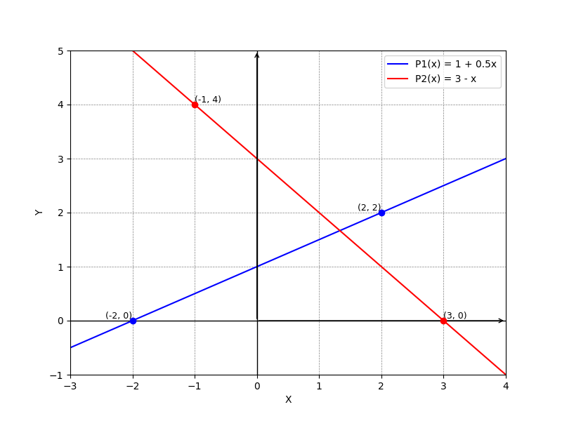
A polynomial can also be uniquely defined by its values at some specific points. For example, two points define a unique line:
- For points and , we have .
- For points and , we have .
Three points define a quadratic polynomial:
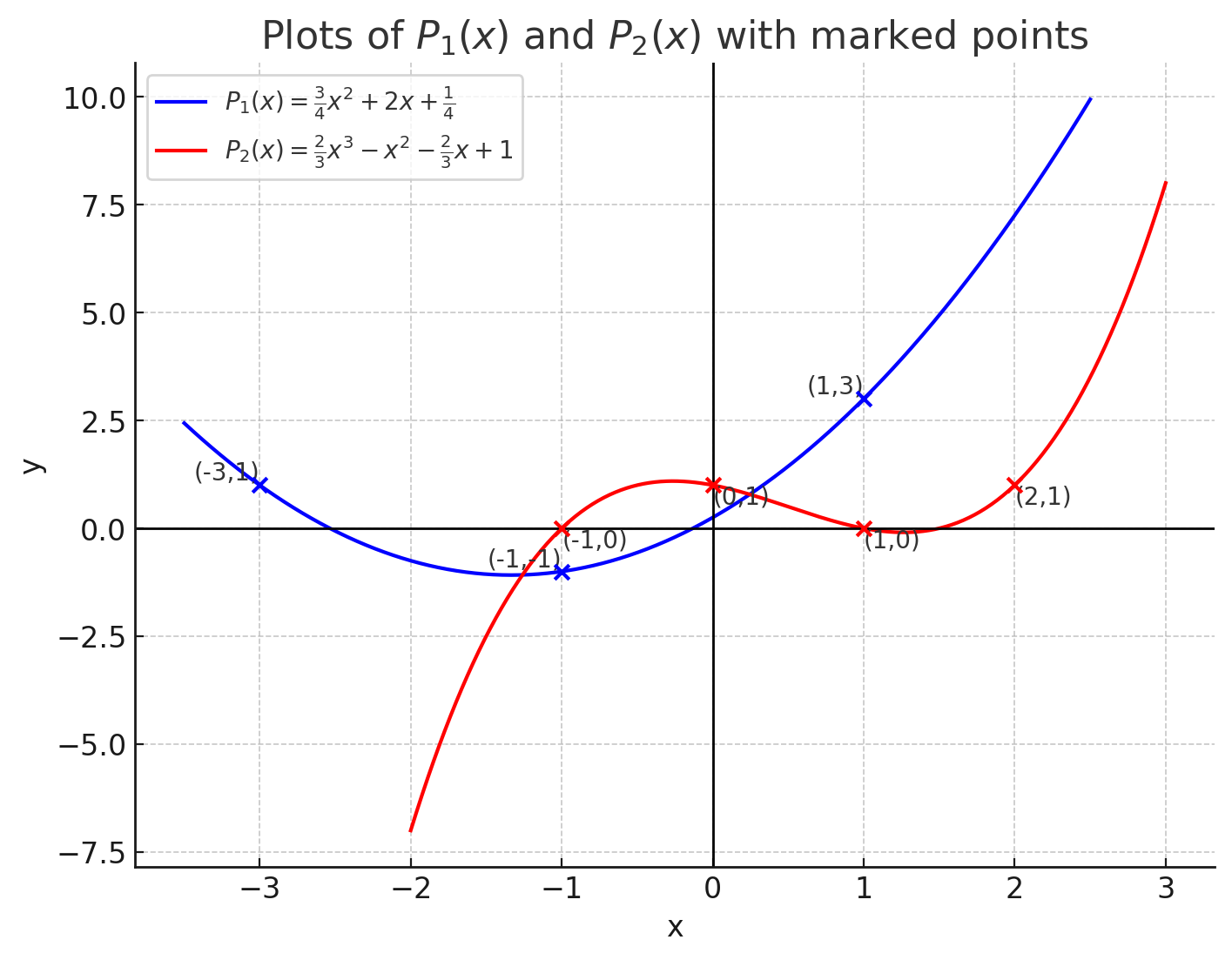
More generally, points uniquely define a polynomial of degree : That is: is invertible for unique Unique exists Unique polynomial exists.
Punchline: Two Unique Trpresentations for Polynomials
Value Representation Advantages
and
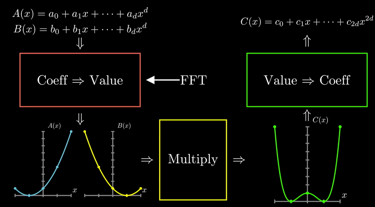
In value representation, multiplication can be performed in linear time rather than quadratic . This is especially advantageous when working with large polynomials.
Polynomial Multiplication Flowchart
Polynomial Evaluation
Evaluation from Coefficients to Values
To evaluate a polynomial at points,we can compute as follows: Howerer, this operation can have a complexity of , which could lead to .
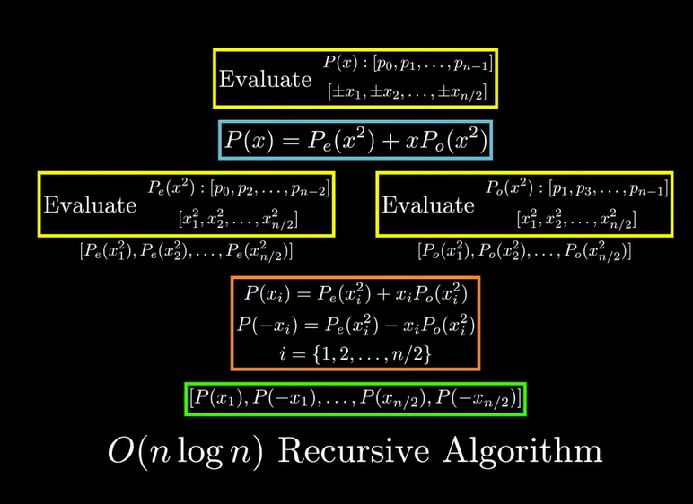
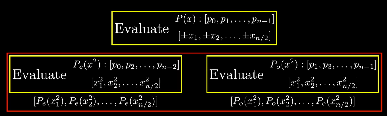
More Efficient Strategies
For example, when evaluatiing at 8 points, we can select symmetric points such as
.
We have .
For we can select:
We have .
So we only need 4 points!
But that is one major problem.
 We can choose the roots of unity in the finite field.
Which Evaluation Points to Use?
To evaluation , we need at least points, ideally for . The points chosen should be the roots of unity:
whers is a root of .
NTT Implementation
def FFT(P):
    # P- [p0,p1,...,p_{n-1}] coeff representation
    n=len(P) # n is a power of 2
    if n==1:
        return P
    w = get_root_of_unity(n)
    P_e,P_o = [P[0],P[2],...,P[n-2]],[P[1],P[3],...,P[n-1]]
    y_e,y_o = FFT(P_e), FFT(P_o)
    y = [0]*n
    for j in range(n/2):
        y[j] = y_e[j]+w^j*y_o[j]
        y[j+n/2] = y_e[j]-w^j*y_o[j]
    return y
Interpolation and Inverse NTT
Alternative Perspective on Evaluation/NTT
That is
Interpolation involves inversing the DFT matrix
The inverse matrix and original matrix look quite similar!
Every in original matrix is now
So the implementation of inverse NTT as follows:
def IFFT(P):
    # P- [p0,p1,...,p_{n-1}] coeff representation
    n=len(P) # n is a power of 2
    if n==1:
        return P
    w = 1/n*(get_root_of_unity(n)^{-1})
    P_e,P_o = [P[0],P[2],...,P[n-2]],[P[1],P[3],...,P[n-1]]
    y_e,y_o = FFT(P_e), FFT(P_o)
    y = [0]*n
    for j in range(n/2):
        y[j] = y_e[j]+w^j*y_o[j]
        y[j+n/2] = y_e[j]-w^j*y_o[j]
    return y